Sensitivity analysis quantifies how changes in an input affect the model output. In risk analysis, it can be used to identify which uncertain inputs are most important for a decision-relevant output. This helps to understand the model behaviour before running it with real data, to prioritise where to intervene to reduce risk, and to increase efforts to reduce uncertainty in the most sensitive inputs.
In mcmodule, you can perform sensitivity analysis using
different methods:
- Scenario (“what-if”) analysis: Compares output changes under targeted input variations, practical for model runs using real data. It does not produce sensitivity indices, but it can be useful for complex models where the most important inputs depend on context.
- Correlation (tornado) analysis: Ranking of influential inputs by correlating each input uncertainty with output uncertainty across existing runs. Only captures inputs that are uncertain in those runs. It can be applied to multivariate inputs, but interpretation can be more complex when correlations vary across variates.
-
Sample design based sensitivity analysis: Evaluates
the model on a predefined input design (e.g., Morris/Sobol) to estimate
sensitivity over a chosen input space using packages such as
sensitivity(Iooss et al. 2025) orsensobol(Puy et al. 2022)and yield sensitivity indices. Inmcmodule, this method is currently limited to one variate.
Scenario analysis
Scenario analysis (or “what-if analysis”) is a non-statistical but still useful approach to assess input sensitivity. It does not produce sensitivity indices, but it will show how the output changes when you make specific changes to the inputs. This makes it a practical way to compare targeted input changes using real input data. It is especially helpful for complex models where the most important inputs depend on context (for example, when estimating disease-entry risk across countries, where certain pathways will be more important in some countries than in others). Scenario analysis can therefore help you identify the most sensitive inputs for a particular use case. This is covered in the working with what-if scenarios section.
Correlation analysis
mcmodule_corr() ranks inputs by their correlation with a
chosen output across the current model runs. It is an extension of
mc2d::tornado() from mc2d (Pouillot and Delignette-Muller
2010) for mcmodule objects and multiple
variates.
Unlike methods that require a sample design, this approach works
directly on an mcmodule built from model input data. Note
that mcmodule_corr() only computes correlations for
uncertain inputs (stochastic nodes built with func) and,
when variates_as_nsv = TRUE, also for multivariate
inputs.
When we correlate specific model input data distributions with outputs, the particular input distributions used in each variate do not necessarily capture the full input sample space. As a result, these correlations indicate where output uncertainty “comes from”, rather than which inputs the output is most sensitive to. A weak correlation does not necessarily mean an input is unimportant (e.g., symmetric non-linear effects can cancel out), and a strong correlation may reflect confounding with other correlated inputs.
Here we compute inputs-output correlations using Spearman coefficient:
# Calculate output (expected number of animals not detected)
imports_mcmodule_corr <- trial_totals(
  imports_mcmodule,
  mc_names = c("no_detect"),
  trials_n = "animals_n",
  subsets_n = "farms_n",
  subsets_p = "h_prev",
  mctable = imports_mctable
)

# Calculate correlations using Spearman's method (default)
corr_results <- mcmodule_corr(imports_mcmodule_corr, output = "no_detect_set_n", method = "spearman")
#>
#> === Correlation Analysis Summary ===
#>
#> Analysis Parameters:
#> - Analysis type: Global output
#> - Output node: no_detect_set_n
#> - Correlation method(s): spearman
#> - Missing value handling: all.obs
#>
#> Expression Information:
#> - Module: mcmodule
#>   - Expression: imports
#>     - Input nodes: w_prev, test_sensi, animals_n, h_prev
#>     - Variates analyzed: 6
#>
#> Results Summary:
#> - Total correlations calculated: 24
#> - Top 4 most influential inputs (by absolute mean correlation):
#>   1. h_prev: 0.7251
#>   2. w_prev: 0.4256
#>   3. animals_n: 0.3073
#>   4. test_sensi: -0.1436
#>
#> Input Correlation Strength Distribution:
#> - Very strong: 2 (8.3%)
#> - Strong: 4 (16.7%)
#> - Moderate: 6 (25.0%)
#> - Weak: 5 (20.8%)
#> - Very weak/None: 7 (29.2%)
#>
#> Inputs by Correlation Strength:
#> - Very strong: h_prev
#> - Strong: w_prev, h_prev, test_sensi
#> - Moderate: animals_n, h_prev, w_prev
#> - Weak: w_prev, animals_n
#> - Very weak/None: test_sensi, animals_n
In this example, h_prev is the main driver of
no_detect_set_n (very strong positive association).
w_prev and animals_n also show positive
correlation, while test_sensi is close to zero or slightly
negative across variates.
# View correlation results
head(corr_results)
#>       exp exp_n variate          output      input        value   method
#> 1 imports     1       1 no_detect_set_n     w_prev  0.685231942 spearman
#> 2 imports     1       1 no_detect_set_n test_sensi  0.004825929 spearman
#> 3 imports     1       1 no_detect_set_n  animals_n  0.461132712 spearman
#> 4 imports     1       1 no_detect_set_n     h_prev  0.511269102 spearman
#> 5 imports     1       2 no_detect_set_n     w_prev  0.268298384 spearman
#> 6 imports     1       2 no_detect_set_n test_sensi -0.016015960 spearman
#>       use   module pathogen origin       strength
#> 1 all.obs mcmodule        a   nord         Strong
#> 2 all.obs mcmodule        a   nord Very weak/None
#> 3 all.obs mcmodule        a   nord       Moderate
#> 4 all.obs mcmodule        a   nord       Moderate
#> 5 all.obs mcmodule        a  south           Weak
#> 6 all.obs mcmodule        a  south Very weak/None
Then visualise the ranking with a tornado plot. It can be customised
with standard ggplot2 layers.
library(ggplot2)
#> Warning: package 'ggplot2' was built under R version 4.5.3

# Plot tornado plot of correlations
mcmodule_tornado(imports_mcmodule_corr, output = "no_detect_set_n", method = "spearman", print_summary = FALSE)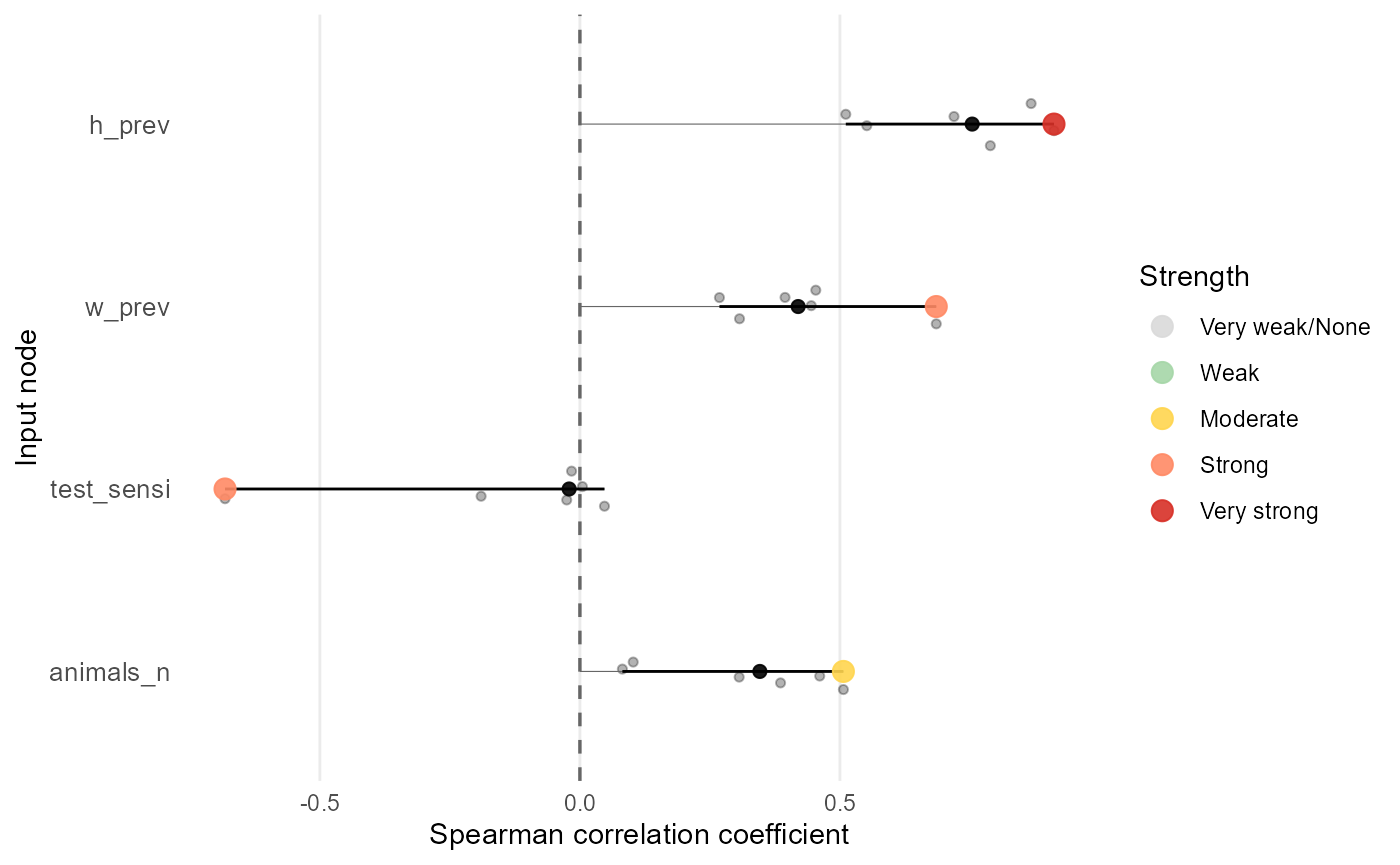
Each point in the plot represents one input variate. The coloured point marks the variate with the largest absolute correlation for that input, and that value is used to rank the inputs. The black point shows the median correlation across variates, which is often a useful summary when correlations vary across the model. The black horizontal line shows the full range of correlations across variates, so you can see whether an input is consistently influential or only influential in certain variates.
Note that farms_n and test_origin are not
shown in this analysis because they are fixed in the original model data
and therefore have zero correlation with the output. This is an
important limitation of correlation-based methods using real input data:
they can only identify influential inputs that vary in the original
model runs. To explore uncertainty for fixed inputs, you need a method
that evaluates a sample design.
Sensitivity analysis with sample design
Create a sample design
An input sample space is the allowable range of values it can take (or distribution definition). A sample design is a specific set of sampled input combinations used to run the model. The sample space defines where values can come from, while the sample design defines which values are actually used in model runs.
A sample_design in mcmodule can be
either:
- a matrix/data frame, or
- a sensitivity object from the
sensitivity::sensitivitypackage (for example, a Morris design object) that has anXelement containing the sampling matrix.
The sampling matrix must have one column per input node and one row per sample. Each row is one scenario in the mcnode uncertainty dimension. When you provide a sample_design, that uncertainty dimension is no longer sampled from the original model inputs; it is mapped to the values in your design. Currently, sample_design supports one variate.
You can pass the sampling matrix (or sensitivity object) directly to
eval_module(), or set it as a global default with
set_sample_design(). Using a global design ensures the same
sampling matrix is available across all model steps, which is convenient
when you run sensitivity analysis after building a complex model. You
can also pass the design to each function call, but that is more
verbose, and you must remove it later to run the model with the original
data inputs.
# Create a sample design as a data frame
X <- data.frame(
  w_prev = runif(10000, 0.15, 0.6),
  h_prev = runif(10000, 0.02, 0.7),
  test_sensi = runif(10000, 0.8, 0.91),
  animals_n = sample(5:10, 10000, replace = TRUE),
  farms_n = sample(82:176, 10000, replace = TRUE),
  test_origin = runif(10000, 0, 1)
)

dim(X)
#> [1] 10000     6
head(X)
#>      w_prev    h_prev test_sensi animals_n farms_n test_origin
#> 1 0.3303008 0.2163915  0.8793875        10      99  0.77421051
#> 2 0.5421882 0.2731196  0.8048914         8     153  0.39541257
#> 3 0.1530968 0.1427685  0.8548849         8      92  0.01832922
#> 4 0.5210398 0.6816595  0.8377471         5     102  0.99870910
#> 5 0.5570636 0.6964915  0.8565773         6     170  0.73319211
#> 6 0.4148973 0.0881092  0.8319424         5     124  0.01512386

# Set global sample design
set_sample_design(X)
#> sample_design set to X

# Retrieve current global sample design
current_design <- set_sample_design()

# Evaluate the module with the global sample design
imports_mcmodule_X <- eval_module(
  exp = imports_exp
)
#> imports_exp evaluated
#> mcmodule created (expressions: imports_exp)

# Calculate output (expected number of animals not detected)
imports_mcmodule_X <- trial_totals(
  imports_mcmodule_X,
  mc_names = c("no_detect"),
  trials_n = "animals_n",
  subsets_n = "farms_n",
  subsets_p = "h_prev"
)

mcmodule_tornado(imports_mcmodule_X, output = "no_detect_set_n", method = "spearman")
#>
#> === Correlation Analysis Summary ===
#>
#> Analysis Parameters:
#> - Analysis type: Global output
#> - Output node: no_detect_set_n
#> - Correlation method(s): spearman
#> - Missing value handling: all.obs
#>
#> Expression Information:
#> - Module: mcmodule
#>   - Expression: imports_exp
#>     - Input nodes: w_prev, test_origin, test_sensi, animals_n, farms_n, h_prev
#>     - Variates analyzed: 1
#>
#> Results Summary:
#> - Total correlations calculated: 6
#> - Top 5 most influential inputs (by absolute mean correlation):
#>   1. h_prev: 0.6743
#>   2. test_origin: -0.4657
#>   3. w_prev: 0.3563
#>   4. animals_n: 0.2211
#>   5. farms_n: 0.2106
#>
#> Input Correlation Strength Distribution:
#> - Very strong: 0 (0.0%)
#> - Strong: 1 (16.7%)
#> - Moderate: 1 (16.7%)
#> - Weak: 3 (50.0%)
#> - Very weak/None: 1 (16.7%)
#>
#> Inputs by Correlation Strength:
#> - Strong: h_prev
#> - Moderate: test_origin
#> - Weak: w_prev, animals_n, farms_n
#> - Very weak/None: test_sensi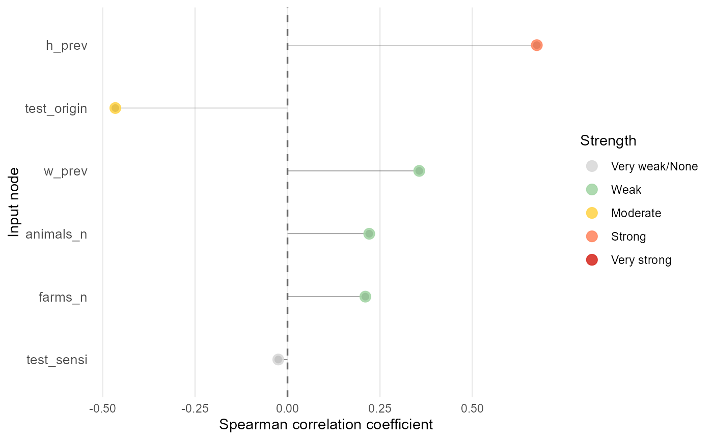
# Reset global sample design
reset_sample_design()
#> sample_design reset
This sample design produces a different ranking from the first
tornado analysis, because we’re using the inputs sampling space rather
than the original model inputs. Here, h_prev is the main
positive driver of no_detect_set_n.
test_origin is the next most influential input and is
negatively associated with the output. w_prev,
animals_n and farms_n have smaller positive
effects, while test_sensi is weak or negligible within
these bounds.
Define sample space in mctable
For methods that use a sample design, mctable can be
used to define how inputs are sampled. In particular,
mctable$sample_space stores the bounds or distribution
parameters used to generate sensitivity samples. To read more about
mctable see the package
vignette.
imports_mctable[,c("mcnode","mc_func", "sample_space")]
#>            mcnode mc_func                        sample_space
#> 1          h_prev   runif               min = 0.02, max = 0.7
#> 2          w_prev   runif               min = 0.15, max = 0.6
#> 3      test_sensi   rpert min = 0.8, mode = 0.875, max = 0.91
#> 4         farms_n    <NA>                   min = 5, max = 10
#> 5       animals_n   rnorm                 min = 82, max = 176
#> 6 test_origin_unk    <NA>                                <NA>
#> 7     test_origin    <NA>                    min = 0, max = 1
Two helper functions support common sampling designs from
mctable:
-
mctable_bounds()for bound (min and max) extraction, for Morris and related approaches. -
mctable_sobol_matrices()for Sobol design matrices.
Currently, mcmodule only provides direct conversion from
mctable to Sobol sampling designs. However, you can use
mctable_bounds() to create many other sample designs using
different approaches. The only requirement is that your sample design
matrix contains columns for all the input nodes in your
mcmodule model.
Morris elementary effects
Morris (Morris 1991) is another screening method. It identifies influential inputs and potential nonlinearity or interactions at moderate computational cost
Start by getting parameter bounds from mctable.
# Get bounds for Morris sampling design
b <- mctable_bounds(imports_mctable, transformation = FALSE)
Build the Morris design with sensitivity::morris(). The
resulting object can be passed directly as sample_design.
The arguments factors, r, and
design control the the factors (inputs) sampled, the number
of repetitions of the design, and the step size between sampled values,
respectively. The arguments binf and bsup
provide the bounds for each input, and scale = TRUE scales
the inputs to [0,1] for better comparability of Morris indices across
inputs with different ranges.
To have stable Morris indices in large sample designs (with many inputs), you need to run the model with a large number of repetitions, which can be computationally intensive. Always check the sensitivity indices stability in diferent runs before interpreting them, increase r until rankings stabilise.
library(sensitivity)
#> Warning: package 'sensitivity' was built under R version 4.5.2
#> Registered S3 method overwritten by 'sensitivity':
#>   method    from
#>   print.src dplyr

# Create Morris design
morris_sa <- sensitivity::morris(
  model = NULL,
  factors = b$factors,
  r = 2000,
  design = list(type = "oat", levels = 4, grid.jump = 2),
  binf = b$binf,
  bsup = b$bsup,
  scale = TRUE
)

# Evaluate the module with that design.
imports_mcmodule_morris <- eval_module(
  exp = imports_exp,
  sample_design = morris_sa,
  mctable = imports_mctable
)
#> imports_exp evaluated
#> mcmodule created (expressions: imports_exp)

# Calculate output (expected number of animals not detected)
imports_mcmodule_morris <- trial_totals(
  imports_mcmodule_morris,
  mc_names = c("no_detect"),
  trials_n = "animals_n",
  subsets_n = "farms_n",
  subsets_p = "h_prev",
  sample_design = morris_sa,
  mctable = imports_mctable
)
Finally, extract the output vector and estimate Morris indices. The
tell() function updates the Morris object with the model
output, and then you can print and plot the indices.
# Extract the output vector and estimate Morris indices.
y <- unmc(imports_mcmodule_morris$node_list$no_detect_set_n$mcnode)

# Aggregated output used for sensitivity analysis.
sensitivity::tell(morris_sa, y)

# Print Morris indices
morris_sa
#>
#> Call:
#> sensitivity::morris(model = NULL, factors = b$factors, r = 2000,     design = list(type = "oat", levels = 4, grid.jump = 2), binf = b$binf,     bsup = b$bsup, scale = TRUE)
#>
#> Model runs: 14000
#>                      mu    mu.star     sigma
#> h_prev       145.607480 145.607480 128.94591
#> w_prev        90.396229  90.396229  99.21655
#> test_sensi    -7.550827   7.550827  10.90713
#> farms_n       50.545247  50.545247  63.27238
#> animals_n     54.153282  54.153282  67.26521
#> test_origin -113.132011 113.132011 113.37709

# Plot Morris indices (mu.star and sigma)
plot(morris_sa)
In the Morris method, mu (
) is the mean of the elementary effects across trajectories and
mu.star (
) is the absolute value of mu, which summarises each
input’s overall importance (larger values indicate a stronger average
influence on the output, regardless of direction). h_prev
has the largest mu.star, making it the most influential
input overall, followed by test_origin. w_prev
is the next most important, while farms_n and
animals_n have more moderate effects, and
test_sensi is negligible within the explored bounds (note
that the uncertainty is small, 0.875-0.91). sigma (
) is the standard deviation of the elementary effects. Large
sigma values indicate that the effect of an input varies
substantially across the sampled space, which typically reflects
nonlinearity and/or interactions with other inputs.
Sobol indices
Sobol analysis Saltelli (2002) decomposes output variance into first-order and higher-order effects, providing a global sensitivity analysis. It is more computationally intensive than Morris, but it gives a more complete picture of input importance, including interactions. Sobol variance decomposition assumes independent inputs, if inputs are dependent, interpret Sobol indices with care or consider other approaches.
First, generate Sobol sampling matrices from
mctable.
mctable_sobol_matrices() creates Sobol design matrices
from your mctable definitions.
library(sensobol)
#> Warning: package 'sensobol' was built under R version 4.5.2

N <- 10000
X <- mctable_sobol_matrices(imports_mctable, N = N, order = "second")
Evaluate the module, compute the target output as before.
imports_mcmodule_sobol <- eval_module(
  exp = imports_exp,
  data = NULL,
  sample_design = X,
  mctable = imports_mctable
)
#> imports_exp evaluated
#> mcmodule created (expressions: imports_exp)

imports_mcmodule_sobol <- trial_totals(
  mcmodule = imports_mcmodule_sobol,
  mc_names = c("no_detect"),
  trials_n = "animals_n",
  subsets_n = "farms_n",
  subsets_p = "h_prev",
  sample_design = X,
  mctable = imports_mctable
)
Then compute first-order (Si) and total-order
(Ti) Sobol indices and print and plot the results.
y <- unmc(imports_mcmodule_sobol$node_list$no_detect_set_n$mcnode)

# Compute Sobol indices
sobol_sa <- sensobol::sobol_indices(Y = y, N = N, params = colnames(X), order = "second", boot = TRUE, R = 1000)

sobol_sa
#>
#> First-order estimator: saltelli | Total-order estimator: jansen
#>
#> Total number of model runs: 230000
#>
#> Sum of first order indices: 0.7854101
#>          original          bias    std.error        low.ci      high.ci
#>             <num>         <num>        <num>         <num>        <num>
#>  1:  3.332841e-01  3.079403e-04 1.503824e-02  0.3035017566 0.3624505639
#>  2:  1.377370e-01  1.216674e-04 1.008885e-02  0.1178415390 0.1573891222
#>  3:  3.909247e-04  8.325475e-06 5.248177e-04 -0.0006460247 0.0014112231
#>  4:  4.305921e-02 -2.350554e-04 5.982279e-03  0.0315692145 0.0550193181
#>  5:  4.684154e-02  2.187586e-04 6.038247e-03  0.0347880384 0.0584575324
#>  6:  2.240974e-01 -1.565078e-04 1.286427e-02  0.1990403770 0.2494673731
#>  7:  4.907211e-01  5.025665e-04 1.219720e-02  0.4663124882 0.5141246176
#>  8:  2.289120e-01  1.673289e-04 6.445115e-03  0.2161124896 0.2413768773
#>  9:  7.520003e-04  1.393999e-06 3.146156e-05  0.0006889428 0.0008122698
#> 10:  7.602997e-02  7.673236e-05 2.190516e-03  0.0716599066 0.0802465711
#> 11:  9.089470e-02  2.012852e-05 2.823745e-03  0.0853401292 0.0964090048
#> 12:  3.490372e-01  1.392118e-04 9.335173e-03  0.3306014041 0.3671946103
#> 13:  4.242323e-02 -2.959331e-04 7.305362e-03  0.0284009199 0.0570374110
#> 14:  2.276340e-04 -1.153166e-05 4.053279e-04 -0.0005552625 0.0010335938
#> 15:  1.158978e-02 -1.286653e-04 4.101202e-03  0.0036802365 0.0197566540
#> 16:  1.559113e-02 -4.948422e-05 4.275080e-03  0.0072616098 0.0240196139
#> 17:  6.621890e-02 -3.910345e-04 8.428252e-03  0.0500908676 0.0831290096
#> 18:  1.986587e-05  4.527382e-07 2.625819e-04 -0.0004952379 0.0005340642
#> 19:  4.869421e-03 -1.756925e-05 2.875823e-03 -0.0007495196 0.0105235003
#> 20:  5.898327e-03  5.359798e-05 2.901685e-03  0.0001575315 0.0115319275
#> 21:  3.005418e-02  3.816841e-05 6.179457e-03  0.0179044955 0.0421275205
#> 22: -5.842551e-06 -3.201330e-07 1.363724e-04 -0.0002728074 0.0002617625
#> 23:  4.855472e-05  8.994252e-06 1.657549e-04 -0.0002853132 0.0003644341
#> 24: -1.751435e-05 -9.576926e-06 3.829174e-04 -0.0007584418 0.0007425670
#> 25:  2.403328e-03  2.890967e-05 1.662343e-03 -0.0008837147 0.0056325520
#> 26:  7.210102e-03 -1.342971e-04 3.452557e-03  0.0005775104 0.0141112870
#> 27:  8.240894e-03 -3.595700e-05 3.808519e-03  0.0008122914 0.0157414100
#>          original          bias    std.error        low.ci      high.ci
#>             <num>         <num>        <num>         <num>        <num>
#>     sensitivity             parameters
#>          <char>                 <char>
#>  1:          Si                 h_prev
#>  2:          Si                 w_prev
#>  3:          Si             test_sensi
#>  4:          Si                farms_n
#>  5:          Si              animals_n
#>  6:          Si            test_origin
#>  7:          Ti                 h_prev
#>  8:          Ti                 w_prev
#>  9:          Ti             test_sensi
#> 10:          Ti                farms_n
#> 11:          Ti              animals_n
#> 12:          Ti            test_origin
#> 13:         Sij          h_prev.w_prev
#> 14:         Sij      h_prev.test_sensi
#> 15:         Sij         h_prev.farms_n
#> 16:         Sij       h_prev.animals_n
#> 17:         Sij     h_prev.test_origin
#> 18:         Sij      w_prev.test_sensi
#> 19:         Sij         w_prev.farms_n
#> 20:         Sij       w_prev.animals_n
#> 21:         Sij     w_prev.test_origin
#> 22:         Sij     test_sensi.farms_n
#> 23:         Sij   test_sensi.animals_n
#> 24:         Sij test_sensi.test_origin
#> 25:         Sij      farms_n.animals_n
#> 26:         Sij    farms_n.test_origin
#> 27:         Sij  animals_n.test_origin
#>     sensitivity             parameters
#>          <char>                 <char>

plot(sobol_sa)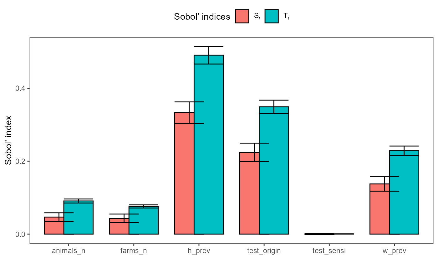
plot(sobol_sa, order = "second")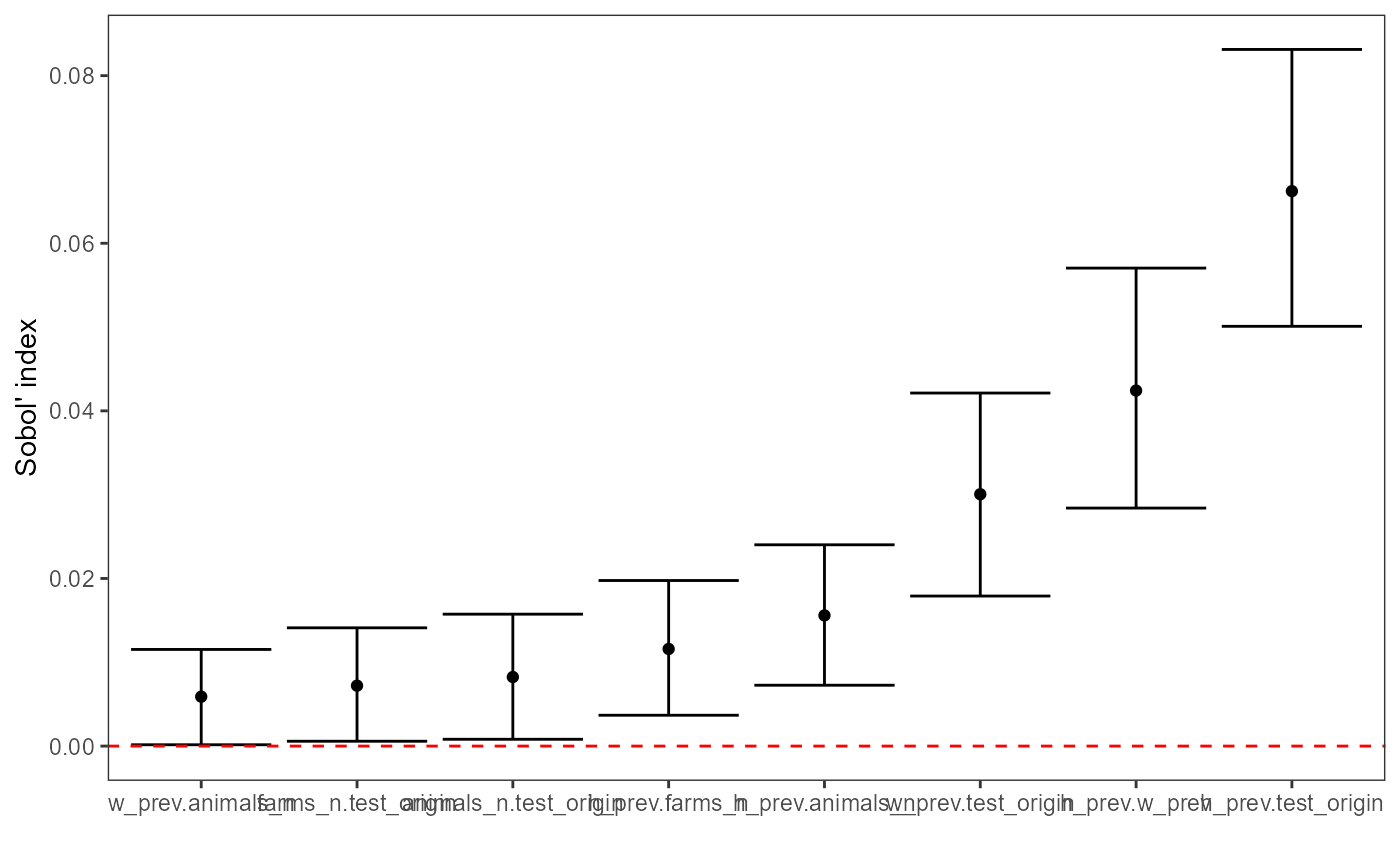
First-order indices (Si) measure each input’s main
effect, the share of output variance attributable to changing that
input alone, averaged over uncertainty in all other inputs. Larger
Si values indicate the model output is more sensitive to
that factor. Here, h_prev is the dominant driver of
variance, test_origin is the next most influential, and
w_prev also contributes materially; farms_n
and animals_n have smaller but non-zero effects, while
test_sensi is negligible. Negative estimates can occur due
to Monte Carlo error and should be interpreted as ~0 if the confidence
interval overlaps 0. If important factors have wide CIs or many
negatives appear, increase N (and/or bootstrap replicates) before
interpreting small effects.
Total-order indices (Ti) measure each input’s total
effect on output variance, including its main effect plus all
interaction effects with other inputs. Ti is therefore
always at least as large as Si for the same parameter.
Second-order indices (Sij) quantify interaction effects.
They measure how much variance is explained only by varying two
inputs together beyond what their individual first-order effects
(Si) explain. Values near 0 indicate little interaction;
larger values indicate the combined effect of the pair is important
(e.g., h_prev.test_origin suggests a meaningful interaction
between h_prev and test_origin).
Other methods
You can use any method to analyse the importance of your inputs as
long as you can build a table/matrix of input values to run the model
with, and collect the corresponding model output(s). For example, you
could use sensitivity::fast99() or Shapley values
(iml::shapley()). The best method will depend on your
model, computational resources, and the specific questions you want to
answer.